Experiment with the Atmosphere
Overview
Teaching: min
Exercises: minQuestions
How do I setup and run an experiment with prescribed ocean forcing?
How is the ocean forcing defined?
Objectives
In this lesson, we will learn about setting up experiments using the atmosphere with the ocean in data mode with prescribed SST forcing.
We will start with a basic case of running an atmosphere-forced experiment. We will then consider a specific scientific question and setup experiments using the atmosphere-forced experiment to answer this question, following the Drought Working Group Experiments.
Running the Atmosphere
Anytime we want to setup a new expeiment, we will create a newcase using the create_newcase script. The script requires us to provide several things when we run it. Let’s figure out the correct options for setting up a case with the atmosphere in forced mode.
--case ~/case/casename
We can name our case whatever we want
--res f19_g17
We are using this resolution, but we will need to check if it is available for what we want to do
--compset COMPSET
We will need to determine the right compset for this experiment.
--project UGMU0032
This is our project code. It does not change.
What compset do we use?
There are two ways to determine which compset to use.
- There is a tool:
$ CIMEROOT/scripts/query_config --compsets
We can see from this that the compsets with cam, the atmosphere model, active all start with F, but it gives us the complicated long name and doesn’t provide us with all the information we need. Let’s take a look at the website for more information.
Notice that the website indicates which version of CESM you are using in the upper right corner. Our version is CESM 2.1.1. Let’s scroll until we find the F compsets.
There are several options here, but the most basic option is FHIST. This is an atmosphere forced run with prescribed ocean and ice using historical GHG forcing.
Remember that the compset determines which grids are scientifically validated, meaning which ones have been tested.
Is our resolution grid
scientifically validatedfor any of theFcompsets?Take a look at the webpage and view the scientifically validated grid for the F-composets. See if our grid is listed.
Create your case
Create a new case using the
FHISTcompset with our grid and project code Call the case whatever you wish.$ ./create_newcase --case ~/cases/testatmF --res f19_g17 --compset FHIST --project UGMU0032You will get an error. Read the error.
What does it mean? What do you need to do to setup your case with this compset and grid resolution?
Solution
create_newcaseis letting us know that our grid is not scientifically validated for this compset. It tells us we can use the--run_unsupportedoption to use this grid and compset anyway.$ ./create_newcase --case ~/cases/testatmF --res f19_g17 --compset FHIST --project UGMU0032 --run-unsupportedComplete the setup, build the case and run it for 1-month as a test
Solution
$ ./case.setup
$ qcmd -- case.build
$ ./xmlchange STOP_OPTION=nmonths
$ ./xmlchange STOP_N=1
How is the ocean prescribed in this run?
Full documentation on DOCN is here
The file specifying the SST and Ice data is located in SSTCE_DATA_FILENAME. We can use xmlquery to see what this is set to.
$ ./xmlquery SSTICE_DATA_FILENAME
SSTICE_DATA_FILENAME: /glade/p/cesmdata/cseg/inputdata/atm/cam/sst/sst_HadOIBl_bc_1x1_1850_2017_c180507.nc
- Let’s look at the description of this variable in
env_run.xml: SSTICE_DATA_FILENAME- Prescribed SST and ice coverage data file name. Sets SST and ice coverage data file name. This is only used when DOCN_MODE=prescribed.
Based on the filename, this appears to be SST and Ice data on a 1x1 degree grid from 1850-2017. We can do ncdump -h on the file to get more information.
$ ncdump -h /glade/p/cesmdata/cseg/inputdata/atm/cam/sst/sst_HadOIBl_bc_1x1_1850_2017_c180507.nc
The data contains several variables: ice_cov, SST_cpl, etc.
The global attributes tell us how this data was made and even give us a reference for it. We can look this up in more detail if we want. For now, let’s take a look at the data using ncview.
$ module load ncview
$ ncview /glade/p/cesmdata/cseg/inputdata/atm/cam/sst/sst_HadOIBl_bc_1x1_1850_2017_c180507.nc
We now know how to create a case with ocean prescribed.
We know how to set the file that prescribes the ocean.
We have an example file that prescribes the ocean.
Key Points
Drought Working Group Experiments
Overview
Teaching: 0 min
Exercises: 0 minQuestions
How do I prescribe my own SSTs to the atmosphere?
Objectives
We will explore this using a set of experiments designed to answer the question of how SSTs in different ocean basins impact drought over the continental US.
History
In 2006, a group of scientists got together to understand predictability of drought because it has such a big societal impact. Each of them had the ability to perform experiments with a different atmosphere model. They put together a set of experiments and each performed the experiment with their own model and they compared the results in the Drought Working Group Paper
The Scientific Question
What is the role of the different ocean basins, including the impact of El Nino–Southern Oscillation (ENSO), the Pacific decadal oscillation (PDO), the Atlantic multidecadal oscillation (AMO), and warming trends in the global oceans in maintining drought from one year to the next?
The Experiments
SST anomalies were defined in the Atlantic and Pacific Oceans based on spatial patterns of annual mean SSTs from 1901-2004 determinedd by rotated EOFS..
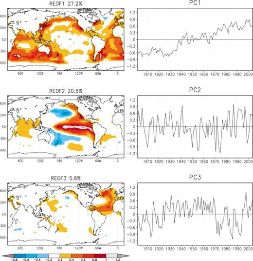 from Schubert et al. Figure 1
The first EOF is consistent with the global mean trend.
The second EOF is concentrated in the Pacific.
The third EOF is concentrated in the Atlantic.
SST anomaly patterns for the Atlantic and Pacific were created based on this analysis. We will look at them later.
A set of 9 experiments consisting of +/- 2 standard deviations in the Atl and Pacific basins and their combinations created 9 base experiments.
| Warm Atlantic | Neutral Atlantic | Cold Atlantic | |
|---|---|---|---|
| Warm Pacific | PwAw | PwAn | PwAc |
| Neutral Pacific | PnAw | PnAn | PnAc |
| Cold Pacific | PcAw | PcAn | PcAc |
They ran the experiments for 50 years and looked at the impact of each combination of SSTs on precipitation anomalies over the continentatl US.
We will reproduce (partially) these experiments as a test of how to setup SST forcing experiments in CESM and evaluate our results.
Key Points
Drought Working Group SSTs
Overview
Teaching: 0 min
Exercises: 0 minQuestions
Setting up the SSTs
Objectives
The SSTs
The SSTs for each experiment are located on COLA in:
/glade/scratch/kpegion/droughtwg/
The SST anomalies for the Pacific are located in: Pacific_SST.nc
The SST anomalies for the Atlantic are located in: N_atl_SST.nc
The climatological SSTs are located in: monthly_climatology_sst_ice.nc
Let’s read in and make a plot of these data. Launch Jupyter (or your preferred Python environment):
An example notebook is located here in: `~kpegion/clim670/droughtwg/droughwgexps.ipynb’. You should copy it to your home directory or any special subdirectory you use for saving class related files:
$ cd
$ cp ~kpegion/clim670/droughtwg/droughwgexps.ipynb .
To launch the Jupyter notebook on the NCAR computers, first login to casper.ucar.edu.
ssh -Y -l username casper.ucar.edu
This is the NCAR data analysis cluster. We use the cheyenne supercomputer to run the model. We use the casper analysis cluster to do data analysis on model output or to do data analysis to prepare data for our model experiments.
Next, we need to load python and activate the python environment:
$ module load python/3.6.8
$ ncar_pylib
Finally, we start Jupyter and follow the instructions on the screen:
$ start-jupyter
Once you start Jupyter you will see the information that tells you to Run the following command on your desktop or laptop: and
The Jupyter web interface will ask you for this token:, followed by a long token of characters.
This token is your Jupyter login information and you should not share it as it could allow others to access your files.
You can now open the Jupyter notebook using the file browser in Jupyter.
We will walk through this notebook to look at our data and then to prepare them for use in the CESM.
- Look at our Drought WG Data
- Look at the CESM SST Data
- Make our Drought WG Data look like CESM SST Data
- Full SST fields (anomalies + climatology)
- Same grid
- Same times
- No missing values
- Same units
-
Make a new SST file for CESM to use
- Replace the right variable with our new SST data.
We can use ncview to take a quick look at our data file and confirm that it looks reasonable.
$ module load ncview
$ ncview /glade/scratch/kpegion/input/dwg_pacpos.nc
Key Points
Run the model with DWG SSTs
Overview
Teaching: 0 min
Exercises: 0 minQuestions
How do I run the model wih these SSTs?
Objectives
Model Configuration
We now need to change the model configuration to run with our new file. We will change some things and confirm a few other configuration parameters
$ ./xmlchange SSTICE_DATA_FILENAME=/glade/scratch/kpegion/input/dwg_pacpos.nc
Check these other variables and confirm we know what they do and how they should be set.
$ ./xmlquery SSTICE_YEAR_START
$ ./xmlquery SSTICE_YEAR_END
$ ./xmlquery SSTICE_YEAR_ALIGN
We will run 1-month as a test.
$ ./xmlchange STOP_N=1
$ ./xmlchange STOP_OPTION=nmonths
$ ./case.submit
Do the SSTs ouput by the model look like your SSTs?
Once your test run is able to run successfully, you will want to cofirm that it is working as expected.
Since yours will have to wait in the queue, we can look at my data to confirm that it ran properly. There is no ocean model output since the ocean is not run.
My data are located in: ‘/glade/scratch/kpegion/archive/testatmF/atm/hist/`
The variable
TSin the atm history files is SST over the ocean. How can you convince youself that the data is consistent enough to believe that the SST data provided is being used by the model?A sample program to get you started is located in:
~kpegion/clim670/CheckSSTData.ipynb
Once we have convinced ourselves that this works properly, how would we continue the run for a full year so we can test that?
Once a full year works and we have tested it properly, how would we run for 10-years?
Key Points
Assignment #3
Overview
Teaching: 0 min
Exercises: 0 minQuestions
What is assignment #3
Objectives
What am I expected to do for Assignment #3
- Run your assigned SST combination from the Drought Working Group for 10 years
P=Pacific; A=Atlantic n = climatology (no SST anomaly) w = 2*SST anomaly c = -2 * SST anomaly
PwAw: Douglas
PwAn: Mary
PwAc: Rachel
PnAw: Hsin
PnAn: Scott
PnAc: Nikki
PcAw: Finley
PcAn: Sherry, Zack
PcAc: Bradley, Joshi
Climatology: Kathy
-
When your data is ready, tell the class where to find it. I will do the same for the climatology experiment.
-
Make a plot of the difference between the annual mean for your experiment and the climatology experiment for precipitation and surface temperature over the continental US for each experiment. This will make 2 9-panel figures. One for preciptiation and one for surface temperature.
To turn in the assignemnt
Point me to the location of your figures/notebook or send me your figure. Due: Oct 27
Key Points