Getting and Reading Data for Today's Class

Overview

Teaching: 0 min
Exercises: 0 min

Questions

How do I find and read in the data for today’s class?

What is an xarray.Dataset?

Objectives

Getting Started

Launch a Jupyter notebook on a COLA server. As a reminder, its best to launch it from your home directory, then you can get to any other directory from within your notebook.
Create a new notebook and save it as Subsetting.ipynb
Import the standard set of packages we use:

import xarray as xr
import numpy as np
import cartopy.crs as ccrs
import matplotlib.pyplot as plt

Find our Dataset

Today we will work with datasets that are on the COLA servers and findable using the COLA Data Catalog. We will start by using monthly Sea Surface Temperature (SST) data.

Go to the COLA Data Catalog

Browse the main catalog and follow the links to obs->gridded->ocn->sst->oisstv2_monthly

Let’s take a look at our dataset and what we can learn about it from the catalog:

It is 1deg x 1deg
Latitudes go from 89.5N to 89.5S – that seems backwards
It goes from Dec 1981 to Apr 2020
It was last updated on the COLA Servers on Jun 25, 2020
It is located in the ‘/shared/obs/gridded/OISSTv2` directory

Now we will take a look at the data on COLA by opening a terminal in our Jupyter Notebook and looking in the directory wehere the data are located:

$ ls /shared/obs/gridded/OISSTv2

lmask  monthly  weekly

Since we are looking for monthly data, let’s look in the monthly sub-directory. Remember, you can use the up-arrow to avoid having to re-type:

$ ls /shared/obs/gridded/OISSTv2/monthly

sst.mnmean.nc

Quick look at Metadata for our Dataset

What command can you use to look at the metadata for our dataset and confirm that it matches the COLA Data Catalog?
Solution
ncdump -h /shared/obs/gridded/OISSTv2/monthly/sst.mnmean.nc

We can now use cut and paste to put the file and directory information into our notebook and read our dataset using xarray

file='/shared/obs/gridded/OISSTv2/monthly/sst.mnmean.nc'
ds=xr.open_dataset(file)
ds

When we run our cells, we get output that looks exactly like the COLA Data Catalog and the results from ncdump -h

It tells us that we have an xarray.Dataset and gives us all the metadata associated with our data.

What is an `xarray.Dataset`?

In climate data analysis, we typically work with multidimensional data. By multidimensional data (also often called N-dimensional), I mean data with many independent dimensions or axes. For example, we might represent Earth’s surface temperature T as a three dimensional variable:

T(x,y,t)

where x is longitude, y is latitude, and t is time.

N-dimensional Data Schematic

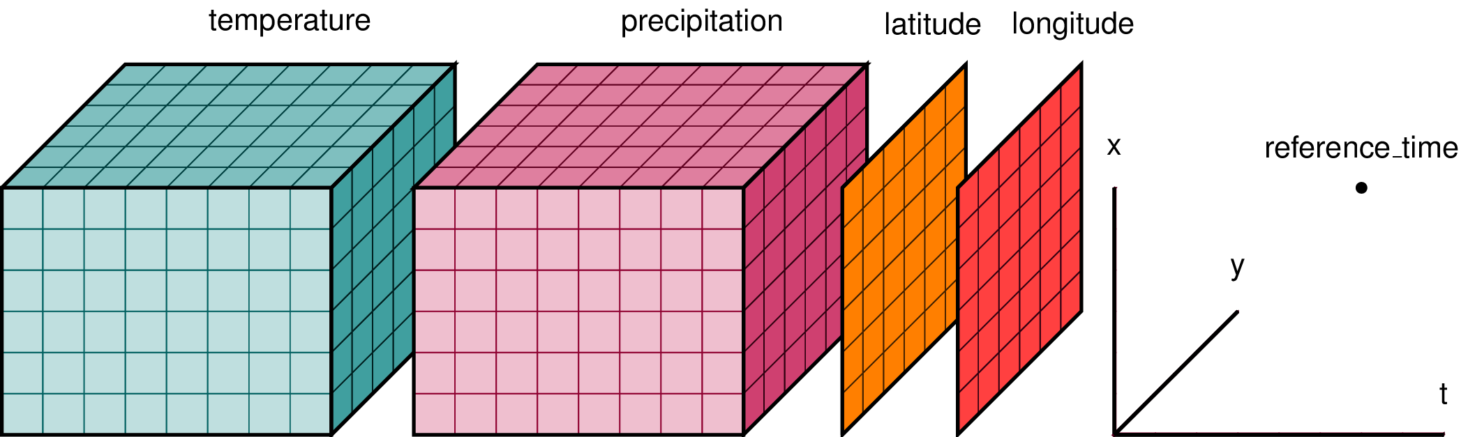
Xarray has two data structures:

a DataArray which holds a single multi-dimensional variable and its coordinates
a Dataset which can hold multiple variables that potentially share the same coordinates

When we read in our data using xr.open_dataset, we read it in as an xr.Dataset.

A DataArray contains:

values: a numpy.ndarray holdy the array’s values
dims: dimension names for each axis (e.g. lon,lat,lev,time)
coords: a container of arrays that label each point
attrs: a container of arbitrary metadata

If we access an individual variable within an xarray.Dataset, we have an xarray.DataArray. Here’s an example:

ds['sst']

you will also see this syntax used

ds.sst

Compare the output for the DataArray and the Dataset

We can access individual attribues attrs of our Dataset using the following syntax:

units=ds['sst'].attrs['units']
print(units)

Using xarray.Dataset.attrs to label figures

Given the following lines of code, how would you use attrs to add units to the colorbar and a title to the map based on the units and long_name attributes?
plt.contourf(ds['sst'][0,:,:])
plt.title(FILLINLONGNAMEHERE)
plt.colorbar(label=FILLINUNITSHERE) 

The Xarray package provides many convenient functions and tools for working with N-dimensional datasets. We will learn some of them today.

Key Points

Subsetting Data

Overview

Teaching: 0 min
Exercises: 0 min

Questions

How do I extract a particular region from my data?

How do I extract a specific time slice from my data?

Objectives

Subsetting data in Space

Often in our research, we want to look at a specific region defined by a set of latitudes and longitudes.

Conventional approach

We would have an array, like an numpy.ndarray with 3 dimensions, such as lat,lon,time that contains our data. We would need to write nested loops with if statements to find the indices of the latitudes and longitudes we are looking for and then extract out those data to a new array.

This is slow, and has the potential for mistakes if we get the wrong indices. Our data and metadata are disconnected.

xarray makes it possible for us to keep our data and metadata connected and select data based on the dimensions, so we can tell it to extract a specific lat-lon point or select a specific range of lats and lons using the sel function.

Select a point

Let’s try it for a point. We will pick a latitude and longitude in the middle of the Pacific Ocean.

ds_point=ds.sel(lat=0,lon=180,method='nearest')
ds_point

We now have a new xarray.Dataset with all the times and a single latitude and longitude point. All the metadata is carried around with our new Dataset. We can plot this timeseries and label the x-axis with the time information.

plt.plot(ds_point['time'],ds_point['sst'])

Select a Region

A common region to look at SSTs is the Nino3.4 region. It is defined as 5S-5N; 170W-120W.

Nino Region

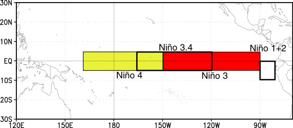
Our longitudes are defined by 0 to 360 (as opposed to -180 to 180), so we need to specify our longitudes consistent with that. To select a region we use the sel command with slice

ds_nino34=ds.sel(lon=slice(360-170,360-120),lat=slice(-5,5))
ds_nino34

Notice that we have no latitudes, what happened? Our data has latitudes going from North to South, but we sliced from South to North. This results in sel finding no latitudes in the range. There are two options to fix this: (1) we can slice in the direction of the latitudes lat=slice(5,-5) or (2) we can reverse the latitudes to go from South to North.

Let’s reverse the latitudes.

ds=ds.reindex(lat=list(reversed(ds['lat'])))

This line reverses the latitudes and then tells xarray to put them back into the latitude coordinate. But, since xarray keeps our metadata attached to our data, we can’t just reverse the latitudes without telling xarray that we want it to attach the reversed latitudes to our data instead of the original latitudes. That’s what the reindex function does.

Now we can slice our data from 5S to 5N

ds_nino34=ds.sel(lon=slice(360-170,360-120),lat=slice(-5,5))
ds_nino34

Now, let’s plot our data

plt.contourf(ds_nino34['lon'],ds_nino34['lat'],
             ds_nino34['sst'][0,:,:],cmap='RdBu_r')
plt.colorbar()

Time Slicing

Sometimes we want to get a particular time slice from our data. Perhaps we have two datasets and we want to select the time slice that is common to both. In this dataset, the data start in Dec 1981 and end in Apr 2020. Suppose we want to extract the times for which we have full years (e.g, Jan 1982 to Dec 2019. We can use the sel function to also select time slices. Let’s select only these times for our ds_nino34 dataset.

ds_nino34=ds_nino34.sel(time=slice('1982-01-01','2019-12-01'))
ds_nino34

Writing data to a file

In this case the dataset is small, but saving off our intermediate datasets is a common step in climate data analysis. This is because our datasets can be very large so we may not want to wait for all our analysis steps to run each time we want to work with this data. We can write out our intermediate data to a file for future use.

It is easy to write an xarray.Dataset to a netcdf file using the to_netcdf() function.

Write out the ds_nino34 dataset to a file in your /scratch directory, like this (replace my username with yours):
ds_nino34.to_netcdf('/scratch/kpegion/nino34_1982-2019.oisstv2.nc')
Bring up a terminal window in Jupyter and convince yourself that the file was written and the metatdata is what you expect by using ncdump

Key Points

Aggregating Data

Overview

Teaching: 0 min
Exercises: 0 min

Questions

How to I aggregate data over various dimensions?

Objectives

The Oceanic Nino Index ONI is used by the Climate Prediction Center to monitor and predict El Nino and La Nina. It is defined as the 3-month running mean of SST anomalies in the Nino3.4 region. We will use aggregation methods from xarray to calculate this index.

First Steps

Create a new notebook and save it as Aggregating.ipynb

Import the standard set of packages we use:

import xarray as xr
import numpy as np
import cartopy.crs as ccrs
import matplotlib.pyplot as plt

Read in the dataset we wrote in the last notebook.

file='/scratch/kpegion/nino34_1982-2019.oisstv2.nc'
ds=xr.open_dataset(file)
ds

Take the mean over a lat-lon region

ds_nino34_index=ds.mean(dim=['lat','lon'])
ds_nino34_index

Our data now has only a time dimension. Make a plot.

plt.plot(ds_nino34_index['time'],ds_nino34_index['sst'])

Calculate Anomalies

Anomaly means departure from normal (called climatology). We often calculate anomalies for working with climate data. We will spend time in a future class learning about calculating climatology and anomalies using another feature of xarray called groupby. Today, I will show you the steps with little explanation.

ds_climo=ds_nino34_index.groupby('time.month').mean()
ds_anoms=ds_nino34_index.groupby('time.month')-ds_climo
ds_anoms

Plot our data.

plt.plot(ds_anoms['time'],ds_anoms['sst'])

Why do I constantly print and plot the data?

Printing the data so I can see its dimensions after each step provides a check on whether my code did what I intended it to do.

Plotting also gives me a quick look to make sure everything makes sense.

I encourage you to do the same when developing and testing new code!

Rolling (Running Means)

The ONI is calculated using a 3-month running mean. This can be done using the rolling function.

Reading and Learning from Documentation

Read the documentation for the xarray.rolling function. Following their example, make a 3-month running mean of the ds_anoms data.
Solution
ds_3m=ds_anoms.rolling(time=3,center=True).mean().dropna(dim='time') 
ds_3m

Let’s plot our original and 3-month running mean data together

plt.plot(ds_anoms['sst'],color='r')
plt.plot(ds_3m['sst'],color='b')
plt.legend(['orig','smooth'])

Some other aggregation functions

There are a number of other aggregate functions such as: std,min,max,sum, among others.

Using the original dataset in this notebook ds, find and plot the maximum SSTs for each gridpoint over the time dimension.
Solution
ds_max=ds.max(dim='time')
plt.contourf(ds_max['sst'],cmap='Reds')
plt.colorbar()
Using the original dataset in this notebook ds, calculate and plot the standard deviation at each gridpoint.
Solution
ds_std=ds.std(dim='time')
plt.contourf(ds_std['sst'],cmap='RdBu_r')
plt.colorbar()

Key Points

Masking

Overview

Teaching: 0 min
Exercises: 0 min

Questions

How to I maskout land or ocean?

Objectives

Sometimes we want to maskout data based on a land/sea mask that is provided.

First Steps

Create a new notebook and save it as Masking.ipynb.

Import the standard set of packages we use:

import xarray as xr
import numpy as np
import cartopy.crs as ccrs
import matplotlib.pyplot as plt

Read in these two datasets:

data_file='/shared/obs/gridded/OISSTv2/monthly/sst.mnmean.nc'
ds_data=xr.open_dataset(data_file)
ds_data

This is the original data file we read in.

mask_file='/shared/obs/gridded/OISSTv2/lmask/lsmask.nc'
ds_mask=xr.open_dataset(mask_file)
ds_mask

Let’s look at this file. It contains a lat-lon grid that is the same as our SST data and a single time. The data are 0’s and 1’s. Plot it.

plt.contourf(ds_mask['mask'])

What does this error mean? The data has a single time dimension so it appears as 3-D to contourf. We can drop single dimensions using squeeze

ds_mask=ds_mask.squeeze()
plt.contourf(ds_mask['mask'])

The latitudes are upside down. Let’s fix that like we did before. In this case, we will fix it for the mask and the data.

ds_mask=ds_mask.reindex(lat=list(reversed(ds_mask['lat'])))
ds_data=ds_data.reindex(lat=list(reversed(ds_data['lat'])))
plt.contourf(ds_mask['mask'])
plt.colorbar()

That’s better! We can see that the mask data are 1 for ocean and 0 for land. We can use xarray.where to mask the data to only over the ocean.

da_ocean=ds_data['sst'].mean('time').where(ds_mask['mask'].squeeze()==1)
da_ocean
plt.contourf(da_ocean,cmap='coolwarm')
plt.colorbar()

Key Points

Interpolating

Overview

Teaching: 0 min
Exercises: 0 min

Questions

How do I interpolate data to a different grid

Objectives

It is common in climate data analysis to need to interpolate data to a different grid. One example is that I have model data on a model grid and observed data on a different grid. I want to calculate a difference between model and obs.

In this lesson, We will make a difference between the average SST in a CMIP5 model historical simulation and the average observed SSTs from the OISSTv2 dataset we have been working with.

Regular Grid

If you are using a regular grid, interpolation is easy using xarray.

A regular grid is one with a 1-dimensional latitude and 1-dimensional longitude. This means that the latitudes are the same for all longitudes and the longitudes are the same for all latitudes.

Most data you encounter will be on a regular grid, but some are not. We will discuss irregular grids in another class.

First Steps

Create a new notebook and save it as Interpolating.ipynb.

Import the standard set of packages we use:

import xarray as xr
import numpy as np
import cartopy.crs as ccrs
import matplotlib.pyplot as plt

Read in obs and mask data:

obs_file='/shared/obs/gridded/OISSTv2/monthly/sst.mnmean.nc'
ds_obs=xr.open_dataset(data_file)
ds_obs

mask_file='/shared/obs/gridded/OISSTv2/lmask/lsmask.nc'
ds_mask=xr.open_dataset(mask_file)
ds_mask

This is the original data file we read in and land/sea mask we previously used.

Remember, we want to reverse the lats

ds_mask=ds_mask.reindex(lat=list(reversed(ds_mask['lat'])))
ds_obs=ds_obs.reindex(lat=list(reversed(ds_obs['lat'])))
plt.contourf(ds_obs['sst'][0,:,:])

Read in the model data

model_path='/shared/cmip5/data/historical/atmos/mon/Amon/ts/NCAR.CCSM4/r1i1p1/'
model_file='ts_Amon_CCSM4_historical_r1i1p1_185001-200512.nc'
ds_model=xr.open_dataset(model_path+model_file)
ds_model

This data has lats from S to N, so we don’t need to reverse it. Take a look at our model data. This data appears to have different units than the obs data.

We can change this.

ds_model['ts']=ds_model['ts']-273.15

Remember that xarray keeps our metadata with our data, so we need to also change the metadata to keep that information correct in our xarray.Dataset

ds_model['ts'].attrs['units']=ds_obs['sst'].attrs['units']

How would you take the time mean of each dataset?

ds_model_mean=ds_model.mean(dim='time')
ds_obs_mean=ds_obs.mean(dim='time')
ds_model_mean

We are now going to use the interp_like function. The documentation tells us that this fucntion interpolates an object onto the coordinates of another object, filling out of range values with NaN.

One important thing to know that is not clear in the documentation is that the coordinates and variable name to interpolate must all be the same.

All variables in the Dataset that have the same name as the one we are interpolating to will be interpolated.

Both of our datasets use lat and lon, but the model dataset uses ts and the obs dataset uses sst. Let’s change the name of the model variable to sst.

ds_model_mean=ds_model_mean.rename({'ts':'sst'})

We will interpolate the model to be like the obs.

model_interp=ds_model_mean.interp_like(ds_obs_mean)
model_interp

Let’s take a look and compare with our data before interpolation.

plt.contourf(model_interp['sst'],cmap='coolwarm')
plt.title('Interpolated')
plt.colorbar()

plt.contourf(ds_model_mean['sst'],cmap='coolwarm')
plt.title('Original')
plt.colorbar()

Now let’s see how different our model mean is from the obs mean. Remember to apply our land/ocean mask.

diff=(model_interp-ds_obs_mean).where(ds_mask['mask'].squeeze()==1)
diff

And plot it…

plt.title('Model - OBS')
plt.contourf(diff['sst'], cmap='coolwarm')
plt.colorbar()

Key Points

Working with Climate Data

Getting and Reading Data for Today's Class

Overview

Getting Started

Find our Dataset

Quick look at Metadata for our Dataset

Solution

What is an xarray.Dataset?

Using xarray.Dataset.attrs to label figures

Key Points

Subsetting Data

Overview

Subsetting data in Space

Conventional approach

Select a point

Select a Region

Time Slicing

Writing data to a file

Key Points

Aggregating Data

Overview

First Steps

Take the mean over a lat-lon region

Calculate Anomalies

Why do I constantly print and plot the data?

Rolling (Running Means)

Reading and Learning from Documentation

Solution

Some other aggregation functions

Solution

Solution

Key Points

Masking

Overview

First Steps

Key Points

Interpolating

Overview

Regular Grid

First Steps

Key Points

What is an `xarray.Dataset`?

Using `xarray.Dataset.attrs` to label figures