Analysis using Xarray
This notebooks demonstrates some features of xarray that are useful for Climate Data Analysis, including:
Reading in multiple files at a time
Averaging over dimensions to calculate an average in space, time, or over ensemble members
Calculating a climatology and anomalies for monthly data
Writing data to netcdf file
Monthly Data
In this notebook, we will work with monthly data as an example.
We will return to the CMIP5 data, this time for surface temperature (ts), which corresponds to sea surface temperature over the ocean, from the RCP4.5 scenario produced by the NCAR/CCSM4 model. This time, we will read in all of the ensemble members at one time.
The data are located on the COLA severs in the following directory: /shared/cmip5/data/rcp45/atmos/mon/Amon/tas/NCAR.CCSM4/r*i1p1/
The filename is: tas_Amon_CCSM4_rcp45_r*i1p1_210101-229912.nc
The ensemble members are indicated by: r1i1p1, r2i1p1, r3i1p1, r4i1p1, r5i1p1, r6i1p1 in the directory and filename.
In xr.open_mfdataset, we can simply use * in the filename and directory name to indicate all the ensemble members.
[1]:
import warnings

import numpy as np
import xarray as xr
import pandas as pd
import matplotlib.pyplot as plt
[2]:
warnings.filterwarnings("ignore")
Read multiple files using xr.open_mfdataset
Set the path and filename using * for the ensemble members
[3]:
path='/shared/cmip5/data/rcp45/atmos/mon/Amon/ts/NCAR.CCSM4/r*i1p1/'
fname='ts_Amon_CCSM4_rcp45_r*i1p1_200601-210012.nc'
Read the data
[4]:
ds=xr.open_mfdataset(path+fname,concat_dim='ensemble',combine='nested',decode_times=True)
print(path+fname)
/shared/cmip5/data/rcp45/atmos/mon/Amon/ts/NCAR.CCSM4/r*i1p1/ts_Amon_CCSM4_rcp45_r*i1p1_200601-210012.nc
When reading the data, we need to tell xarray how to put the data together. Here, I told it to create a new dimension called ensemble for combining the data.
[5]:
ds
[5]:
<xarray.Dataset>
Dimensions:    (bnds: 2, ensemble: 6, lat: 382, lon: 288, time: 1140)
Coordinates:
  * lon        (lon) float64 0.0 1.25 2.5 3.75 5.0 ... 355.0 356.2 357.5 358.8
  * lat        (lat) float64 -90.0 -89.06 -89.06 -88.12 ... 89.06 89.06 90.0
  * time       (time) object 2006-01-16 12:00:00 ... 2100-12-16 12:00:00
Dimensions without coordinates: bnds, ensemble
Data variables:
    time_bnds  (ensemble, time, bnds) object dask.array<chunksize=(1, 1140, 2), meta=np.ndarray>
    lat_bnds   (ensemble, lat, bnds) float64 dask.array<chunksize=(1, 382, 2), meta=np.ndarray>
    lon_bnds   (ensemble, lon, bnds) float64 dask.array<chunksize=(1, 288, 2), meta=np.ndarray>
    ts         (ensemble, time, lat, lon) float32 dask.array<chunksize=(1, 1140, 382, 288), meta=np.ndarray>
Attributes:
    institution:                  NCAR (National Center for Atmospheric Resea...
    institute_id:                 NCAR
    experiment_id:                rcp45
    source:                       CCSM4
    model_id:                     CCSM4
    forcing:                      Sl GHG Vl SS Ds SA BC MD OC Oz AA
    parent_experiment_id:         historical
    parent_experiment_rip:        r1i1p1
    branch_time:                  2005.0
    contact:                      cesm_data@ucar.edu
    references:                   Gent P. R., et.al. 2011: The Community Clim...
    initialization_method:        1
    physics_version:              1
    tracking_id:                  635969e3-0203-402b-a58b-e3630cb58a30
    acknowledgements:             The CESM project is supported by the Nation...
    cesm_casename:                b40.rcp4_5.1deg.001
    cesm_repotag:                 ccsm4_0_beta49
    cesm_compset:                 BRCP45CN
    resolution:                   f09_g16 (0.9x1.25_gx1v6)
    forcing_note:                 Additional information on the external forc...
    processed_by:                 strandwg on mirage0 at 20111021
    processing_code_information:  Last Changed Rev: 428 Last Changed Date: 20...
    product:                      output
    experiment:                   RCP4.5
    frequency:                    mon
    creation_date:                2011-10-21T21:56:36Z
    history:                      2011-10-21T21:56:36Z CMOR rewrote data to c...
    Conventions:                  CF-1.4
    project_id:                   CMIP5
    table_id:                     Table Amon (26 July 2011) 976b7fd1d9e1be31d...
    title:                        CCSM4 model output prepared for CMIP5 RCP4.5
    parent_experiment:            historical
    modeling_realm:               atmos
    realization:                  1
    cmor_version:                 2.7.1
This next step converts the time dimension to a type that can be used later for plotting
[6]:
ds['time'] = pd.to_datetime(ds.time.values.astype(str))
As you can see, the data now has an ensemble dimension of size 6 corresponding to each of our ensemble members.
Calculate the Ensemble Mean
xarray has nice features for performing operations over a specified dimension or set of dimension. One example is xr.mean which we can use to average over the ensemble dimension to make the ensemble mean.
[7]:
ds_emean=ds.mean(dim='ensemble')
[8]:
ds_emean
[8]:
<xarray.Dataset>
Dimensions:   (bnds: 2, lat: 382, lon: 288, time: 1140)
Coordinates:
  * lon       (lon) float64 0.0 1.25 2.5 3.75 5.0 ... 355.0 356.2 357.5 358.8
  * lat       (lat) float64 -90.0 -89.06 -89.06 -88.12 ... 89.06 89.06 90.0
  * time      (time) datetime64[ns] 2006-01-16T12:00:00 ... 2100-12-16T12:00:00
Dimensions without coordinates: bnds
Data variables:
    lat_bnds  (lat, bnds) float64 dask.array<chunksize=(382, 2), meta=np.ndarray>
    lon_bnds  (lon, bnds) float64 dask.array<chunksize=(288, 2), meta=np.ndarray>
    ts        (time, lat, lon) float32 dask.array<chunksize=(1140, 382, 288), meta=np.ndarray>
As you can see, the ensemble dimension is no longer shown, but all the metadata is still present in the xr.Dataset
Calculate Anomalies for Monthly Data
We often want to calculate anomalies for climate data analysis. xarray has a function called groupby which allows us to group the data by months. We can then apply a mean function over the months to get the climatology and subtract that from the original data to get anomalies.
[9]:
ds_climo = ds_emean.groupby('time.month').mean('time')
ds_anoms = (ds_emean.groupby('time.month') - ds_climo)
Let’s convince ourselves that the climatology and anomalies we calculated look like what we expect. We will use xr.sel to select a specific latitude and longitude and plot them. Here, we tell xarray to select the values nearest the latitude and logitude of Fairfax, VA (39N,77W)
[10]:
ds_climopt=ds_climo.sel(lon='283',lat='39',method='nearest')
ds_anomspt=ds_anoms.sel(lon='283',lat='39',method='nearest')
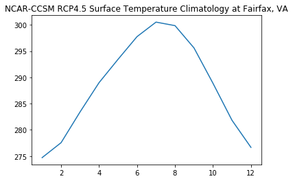
Plot the Climatology
[11]:
plt.plot(ds_climopt['month'],ds_climopt['ts'][0:12])
plt.title('NCAR-CCSM RCP4.5 Surface Temperature Climatology at Fairfax, VA')
[11]:
Text(0.5, 1.0, 'NCAR-CCSM RCP4.5 Surface Temperature Climatology at Fairfax, VA')
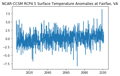
Plot the Anomalies
[12]:
plt.plot(ds_anomspt['time'],ds_anomspt['ts'])
plt.title('NCAR-CCSM RCP4.5 Surface Temperature Anomalies at Fairfax, VA')
[12]:
Text(0.5, 1.0, 'NCAR-CCSM RCP4.5 Surface Temperature Anomalies at Fairfax, VA')
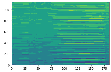
Make Hovmoller Diagram of EQ Pacific SST Anomalies
We will use xarray sel and slice to extract 5S-5N, 60-290 and mean to average over the latitudes
[13]:
eqpac=ds_anoms.sel(lon=slice(60,290),lat=slice(-5,5)).mean(dim='lat')
eqpac
[13]:
<xarray.Dataset>
Dimensions:   (bnds: 2, lon: 185, time: 1140)
Coordinates:
  * lon       (lon) float64 60.0 61.25 62.5 63.75 ... 286.2 287.5 288.8 290.0
  * time      (time) datetime64[ns] 2006-01-16T12:00:00 ... 2100-12-16T12:00:00
    month     (time) int64 1 2 3 4 5 6 7 8 9 10 11 ... 2 3 4 5 6 7 8 9 10 11 12
Dimensions without coordinates: bnds
Data variables:
    lat_bnds  (time, bnds) float64 dask.array<chunksize=(1, 2), meta=np.ndarray>
    lon_bnds  (time, lon, bnds) float64 dask.array<chunksize=(1, 185, 2), meta=np.ndarray>
    ts        (time, lon) float32 dask.array<chunksize=(1, 185), meta=np.ndarray>
[14]:
plt.contourf(eqpac['ts'])
[14]:
<matplotlib.contour.QuadContourSet at 0x7f11a517c978>
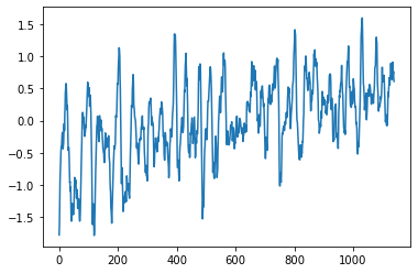
Calculate the Nino3.4 Index
We can use xarray sel, slice, and mean to calculate the Nino3.4 index by taking the mean over multiple dimensions
[15]:
ds_nino34=ds_anoms.sel(lat=slice(-5,5),lon=slice(190,240)).mean(['lat','lon'])
[16]:
plt.plot(ds_nino34['ts'])
[16]:
[<matplotlib.lines.Line2D at 0x7f11a4db2d68>]
Write data to netcdf file
[17]:
ds_nino34.to_netcdf('nino34.nc')