Read a netcdf file and make a contour plot of the data

In this example, we demonstrate: 1. How to read a netcdf file in Python using xarray 2. How to make a contour plot of the data

Data

We will read CMIP5 data for surface air temperature (tas) from the RCP8.5 scenario produced by the NCAR/CCSM4 model. For this example, we will read teh first ensemble member.

The data are located on the COLA severs in the following directory: /shared/cmip5/data/rcp45/atmos/mon/Amon/tas/NCAR.CCSM4/r1i1p1/

The filename is: tas_Amon_CCSM4_rcp45_r1i1p1_210101-229912.nc

Python import statements

You must first import the Python packages you wish to use. This is a common set of basic import statments you can start with.

import numpy as np
import xarray as xr
import matplotlib.pyplot as plt

Set the path and filename

path='/shared/cmip5/data/rcp45/atmos/mon/Amon/tas/NCAR.CCSM4/r1i1p1/'
fname='tas_Amon_CCSM4_rcp45_r1i1p1_200601-210012.nc'

Read the data using xarray open_dataset http://xarray.pydata.org/en/stable/generated/xarray.open_dataset.html

ds=xr.open_dataset(path+fname)

When you read in data using xarray, it creates an object called an xarray.Dataset which consists of your data and all its metadata. If we print out our Dataset which is called ds, its similar to doing a ncdump -h on a netcdf file. You can see all the dimensions, size, and attributes of the data in the file.

ds

<xarray.Dataset>
Dimensions:    (bnds: 2, lat: 192, lon: 288, time: 1140)
Coordinates:
  * time       (time) object 2006-01-16 12:00:00 ... 2100-12-16 12:00:00
  * lat        (lat) float64 -90.0 -89.06 -88.12 -87.17 ... 88.12 89.06 90.0
  * lon        (lon) float64 0.0 1.25 2.5 3.75 5.0 ... 355.0 356.2 357.5 358.8
    height     float64 ...
Dimensions without coordinates: bnds
Data variables:
    time_bnds  (time, bnds) object ...
    lat_bnds   (lat, bnds) float64 ...
    lon_bnds   (lon, bnds) float64 ...
    tas        (time, lat, lon) float32 ...
Attributes:
    institution:                  NCAR (National Center for Atmospheric Resea...
    institute_id:                 NCAR
    experiment_id:                rcp45
    source:                       CCSM4
    model_id:                     CCSM4
    forcing:                      Sl GHG Vl SS Ds SA BC MD OC Oz AA
    parent_experiment_id:         historical
    parent_experiment_rip:        r1i1p1
    branch_time:                  2005.0
    contact:                      cesm_data@ucar.edu
    references:                   Gent P. R., et.al. 2011: The Community Clim...
    initialization_method:        1
    physics_version:              1
    tracking_id:                  0bf35136-b266-44d2-9078-f3081b83b6ad
    acknowledgements:             The CESM project is supported by the Nation...
    cesm_casename:                b40.rcp4_5.1deg.001
    cesm_repotag:                 ccsm4_0_beta49
    cesm_compset:                 BRCP45CN
    resolution:                   f09_g16 (0.9x1.25_gx1v6)
    forcing_note:                 Additional information on the external forc...
    processed_by:                 strandwg on mirage0 at 20111021
    processing_code_information:  Last Changed Rev: 428 Last Changed Date: 20...
    product:                      output
    experiment:                   RCP4.5
    frequency:                    mon
    creation_date:                2011-10-21T21:56:22Z
    history:                      2011-10-21T21:56:22Z CMOR rewrote data to c...
    Conventions:                  CF-1.4
    project_id:                   CMIP5
    table_id:                     Table Amon (26 July 2011) 976b7fd1d9e1be31d...
    title:                        CCSM4 model output prepared for CMIP5 RCP4.5
    parent_experiment:            historical
    modeling_realm:               atmos
    realization:                  1
    cmor_version:                 2.7.1

If you want to access just the surface air tempeature (tas) data itself, without all the gloal attributes, you can do that by supplying the name of the variable

ds['tas']

<xarray.DataArray 'tas' (time: 1140, lat: 192, lon: 288)>
[63037440 values with dtype=float32]
Coordinates:
  * time     (time) object 2006-01-16 12:00:00 ... 2100-12-16 12:00:00
  * lat      (lat) float64 -90.0 -89.06 -88.12 -87.17 ... 87.17 88.12 89.06 90.0
  * lon      (lon) float64 0.0 1.25 2.5 3.75 5.0 ... 355.0 356.2 357.5 358.8
    height   float64 ...
Attributes:
    standard_name:     air_temperature
    long_name:         Near-Surface Air Temperature
    units:             K
    original_name:     TREFHT
    comment:           TREFHT no change
    cell_methods:      time: mean (interval: 30 days)
    cell_measures:     area: areacella
    history:           2011-10-21T21:56:22Z altered by CMOR: Treated scalar d...
    associated_files:  baseURL: http://cmip-pcmdi.llnl.gov/CMIP5/dataLocation...

Let’s make a very simple contour plot to convince ourselves that we indeed have surface air temperature data. 1. We will use the matplotlib plt.contourf function for a filed contour plot. It works very similar to Matlab plotting functions.

2. We can only make a contour plot with 2-D data (lat,lon) and we have 3-D (time,lat,lon), so we will need to access a single time using brackets notation. 3. We will want to add a colorbar to see that values are reasonable

plt.contourf(ds['tas'][0,:,:])
plt.colorbar()

<matplotlib.colorbar.Colorbar at 0x7f95fc109c88>

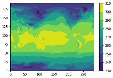
This is a very simple plot, but it looks like we have global temperature data. More details on how to plot maps, make nice lables, and colors, can be found in other examples.