Calculate ENSO Skill as a Function of Initial Month vs. Lead Time¶

In this example, we demonstrate:¶

How to remotely access data from the North American Multi-model Ensemble (NMME) hindcast database and set it up to be used in climpred.
How to calculate the Anomaly Correlation Coefficient (ACC) using monthly data
How to calculate and plot historical forecast skill of the Nino3.4 index as function of initialization month and lead time.

The North American Multi-model Ensemble (NMME)¶

Further information on NMME is available from Kirtman et al. 2014 and the NMME project website

The NMME public database is hosted on the International Research Institute for Climate and Society (IRI) data server http://iridl.ldeo.columbia.edu/SOURCES/.Models/.NMME/

Since the NMME data server is accessed via this notebook, the time for the notebook to run may take a few minutes and vary depending on the speed that data is downloaded.

Definitions¶

Anomalies: Departure from normal, where normal is defined as the climatological value based on the average value for each month over all years.
Nino3.4: An index used to represent the evolution of the El Nino-Southern Oscillation (ENSO). Calculated as the average sea surface temperature (SST) anomalies in the region 5S-5N; 190-240

[1]:

import warnings

import matplotlib.pyplot as plt
import xarray as xr
import pandas as pd
import numpy as np
from tqdm.auto import tqdm

from climpred import HindcastEnsemble
import climpred

[2]:

warnings.filterwarnings("ignore")

Function to set 360 calendar to 360_day calendar and decond cf times

[3]:

def decode_cf(ds, time_var):
    if ds[time_var].attrs['calendar'] == '360':
        ds[time_var].attrs['calendar'] = '360_day'
    ds = xr.decode_cf(ds, decode_times=True)
    return ds

Load the monthly sea surface temperature (SST) hindcast data for the NCEP-CFSv2 model from the NMME data server. This is a large dataset, so we allow dask to chunk the data as it chooses.

[4]:

url = 'http://iridl.ldeo.columbia.edu/SOURCES/.Models/.NMME/NCEP-CFSv2/.HINDCAST/.MONTHLY/.sst/dods'
fcstds = decode_cf(xr.open_dataset(url, decode_times=False,
                                   chunks={'S': 'auto', 'L': 'auto', 'M':'auto'}),'S')

fcstds

[4]:

<xarray.Dataset>
Dimensions:  (L: 10, M: 24, S: 348, X: 360, Y: 181)
Coordinates:
  * S        (S) object 1982-01-01 00:00:00 ... 2010-12-01 00:00:00
  * M        (M) float32 1.0 2.0 3.0 4.0 5.0 6.0 ... 20.0 21.0 22.0 23.0 24.0
  * X        (X) float32 0.0 1.0 2.0 3.0 4.0 ... 355.0 356.0 357.0 358.0 359.0
  * L        (L) float32 0.5 1.5 2.5 3.5 4.5 5.5 6.5 7.5 8.5 9.5
  * Y        (Y) float32 -90.0 -89.0 -88.0 -87.0 -86.0 ... 87.0 88.0 89.0 90.0
Data variables:
    sst      (S, L, M, Y, X) float32 dask.array<chunksize=(6, 5, 8, 181, 360), meta=np.ndarray>
Attributes:
    Conventions:  IRIDL

The NMME data dimensions correspond to the following climpred dimension definitions: X=lon,L=lead,Y=lat,M=member, S=init. We will rename the dimensions to their climpred names.

[5]:

fcstds=fcstds.rename({'S': 'init','L': 'lead','M': 'member', 'X': 'lon', 'Y': 'lat'})

Let’s make sure that the lead dimension is set properly for climpred. NMME data stores leads as 0.5, 1.5, 2.5, etc, which correspond to 0, 1, 2, … months since initialization. We will change the lead to be integers starting with zero. climpred also requires that lead dimension has an attribute called units indicating what time units the lead is assocated with. Options are: years,seasons,months,weeks,pentads,days. For the monthly NMME data, the lead units are months.

[6]:

fcstds['lead']=(fcstds['lead']-0.5).astype('int')
fcstds['lead'].attrs={'units': 'months'}

Now we need to make sure that the init dimension is set properly for climpred. For monthly data, the init dimension must be a xr.cfdateTimeIndex or a pd.datetimeIndex. We convert the init values to pd.datatimeIndex.

[7]:

fcstds['init']=pd.to_datetime(fcstds.init.values.astype(str))
fcstds['init']=pd.to_datetime(fcstds['init'].dt.strftime('%Y%m01 00:00'))

Next, we want to get the verification SST data from the data server

[8]:

obsurl='http://iridl.ldeo.columbia.edu/SOURCES/.Models/.NMME/.OIv2_SST/.sst/dods'
verifds = decode_cf(xr.open_dataset(obsurl, decode_times=False),'T')
verifds

[8]:

<xarray.Dataset>
Dimensions:  (T: 405, X: 360, Y: 181)
Coordinates:
  * Y        (Y) float32 -90.0 -89.0 -88.0 -87.0 -86.0 ... 87.0 88.0 89.0 90.0
  * X        (X) float32 0.0 1.0 2.0 3.0 4.0 ... 355.0 356.0 357.0 358.0 359.0
  * T        (T) object 1982-01-16 00:00:00 ... 2015-09-16 00:00:00
Data variables:
    sst      (T, Y, X) float32 ...
Attributes:
    Conventions:  IRIDL

Rename the dimensions to correspond to climpred dimensions

[9]:

verifds=verifds.rename({'T': 'time','X': 'lon', 'Y': 'lat'})

Convert the time data to be of type pd.datetimeIndex

[10]:

verifds['time']=pd.to_datetime(verifds.time.values.astype(str))
verifds['time']=pd.to_datetime(verifds['time'].dt.strftime('%Y%m01 00:00'))

Subset the data to 1982-2010

[11]:

fcstds=fcstds.sel(init=slice('1982-01-01','2010-12-01'))
verifds=verifds.sel(time=slice('1982-01-01','2010-12-01'))

Calculate the Nino3.4 index for forecast and verification.

[12]:

fcstnino34=fcstds.sel(lat=slice(-5,5),lon=slice(190,240)).mean(['lat','lon'])
verifnino34=verifds.sel(lat=slice(-5,5),lon=slice(190,240)).mean(['lat','lon'])

fcstclimo = fcstnino34.groupby('init.month').mean('init')
fcst = (fcstnino34.groupby('init.month') - fcstclimo)

verifclimo = verifnino34.groupby('time.month').mean('time')
verif = (verifnino34.groupby('time.month') - verifclimo)

Because will will calculate the anomaly correlation coefficient over all time for verification and init for the hindcasts, we need to rechunk the data so that these dimensions are in same chunk

[13]:

fcst=fcst.chunk({'init':-1})
verif=verif.chunk({'time':-1})

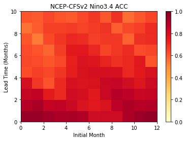
Use the climpred HindcastEnsemble to calculate the anomaly correlation coefficient (ACC) as a function of initial month and lead

[14]:

skill=np.zeros((fcst['lead'].size, 12))
for im in tqdm(np.arange(0,12)):
    hindcast = HindcastEnsemble(fcst.sel(init=fcst['init.month']==im+1))
    hindcast = hindcast.add_observations(verif, 'observations')
    skillds = hindcast.verify(metric='acc')
    skill[:,im]=skillds['sst'].values

Plot the ACC as function of Initial Month and lead-time

[15]:

plt.pcolormesh(skill,cmap=plt.cm.YlOrRd,vmin=0.0,vmax=1.0)
plt.colorbar()
plt.title('NCEP-CFSv2 Nino3.4 ACC')
plt.xlabel('Initial Month')
plt.ylabel('Lead Time (Months)')

[15]:

Text(0, 0.5, 'Lead Time (Months)')

../_images/examples_monthly-enso-subx-example_31_1.png

References¶

Kirtman, B.P., D. Min, J.M. Infanti, J.L. Kinter, D.A. Paolino, Q. Zhang, H. van den Dool, S. Saha, M.P. Mendez, E. Becker, P. Peng, P. Tripp, J. Huang, D.G. DeWitt, M.K. Tippett, A.G. Barnston, S. Li, A. Rosati, S.D. Schubert, M. Rienecker, M. Suarez, Z.E. Li, J. Marshak, Y. Lim, J. Tribbia, K. Pegion, W.J. Merryfield, B. Denis, and E.F. Wood, 2014: The North American Multimodel Ensemble: Phase-1 Seasonal-to-Interannual Prediction; Phase-2 toward Developing Intraseasonal Prediction. Bull. Amer. Meteor. Soc., 95, 585–601, https://doi.org/10.1175/BAMS-D-12-00050.1